12. SciPy重心拉格郎日插值
拉格朗日插值法的公式结构整齐紧凑,在理论分析中十分方便,然而在计算中,当插值点增加或减少一个时,所对应的基本多项式就需要全部重新计算,于是整个公式都会变化,非常繁琐。这时可以用重心拉格朗日插值法或牛顿插值法来代替。此外,当插值点比较多的时候,拉格朗日插值多项式的次数可能会很高,因此具有数值不稳定的特点。 Barycentric Lagrange Interpolation即重心坐标拉格郎日插值,是Jean-Paul Berrut 与 Lloyd N. Trefethen共同提出的对经典拉格郎日插值算法的改进、增强版,有效地克服一般插值方法的振荡性和向前性,具有计算精度高、不用划分网格、程序易实现等诸多优点,且当插值点较大时仍具有良好的数值稳定性。
12.1 重心拉格朗日插值公式
设集合$D_n=${$0,1,\cdots,n$},$B_k = ${$\;i\;\vert\; i \neq k\;,i \in D_n$},对于任意$\;k \in D_n$得到拉格朗日基本多项式(插值基函数)公式:拉格朗日基本多项式(插值基函数)公式: $$ P_k(x) = \prod_{i \in B_k} \frac{x-x_i}{x_k - x_i} = \frac{\prod_{i \in B_k} x - x_i}{\prod_{i \in B_k} x_k-x_i} $$ 拉格朗日插值多项式: $$ L_n(x)=\sum_{j = 0}^{n}y_jP_j(x) $$ 令: $$ \ell(x) = \prod_{i = 0}^{n}(x - x_i) $$ $$ \omega_k =\frac{1}{\prod_{i \in B_k}(x_k - x_i)} $$ 存在: $$ \omega_k = \frac{1}{\ell'(x_k)} $$ $$ \prod_{i \in B_k}(x - x_i) = \frac{\ell(x)}{x - x_k} $$ 因此: $$ \Longrightarrow P_k(x) = \frac{\ell(x)}{x - x_i}\times \frac{1}{\prod_{i \in B_k}(x_k - x_i)} =\ell(x) \frac{\omega_k}{x - x_k} $$ $$ \Longrightarrow L_n(x) = \sum_{j = 0}^{n}y_jP_j(x) = \ell(x)\sum_{j = 0}^{n}y_j\frac{\omega_j}{x - x_j} $$ 对于$\forall x \in R$存在函数$g(x)\equiv1$进行拉格郎日插值,可以得到: $$ 1\equiv g(x) = \ell(x)\sum_{j = 0}^{n}y_j\frac{\omega_j}{x - x_j}\quad,\;y_i = 1 $$ 两式相除: $$ \frac{L_n(x)}{g(x)} = L_n(x) = \frac{\sum_{j = 0}^{n}\frac{\omega_j}{x - x_j}y_j}{\sum_{j = 0}^{n}\frac{\omega_j}{x - x_j}} $$ 这个公式被称为重心拉格朗日插值公式。
12.2 使用重心插值
下面以$f(x)$是一个通过3个点的$x$的二次多项式,来验证一下重心拉格朗日插值公式,假设有三个点(1,3)、(2,7)、(3,13)得$x_0=1,x_1=2,x_2= 3$和$y_0 = 3,y_1 = 7,y_2 =13$: $$f(x) = L_n(x)= \frac{\sum_{j = 0}^{n}\frac{\omega_j}{x - x_j}y_j}{\sum_{j = 0}^{n}\frac{\omega_j}{x - x_j}}$$ 1). 先计算$\omega_i\;i\in(0,1,2)$: $$ \omega_0 = \frac{1}{(x_0 - x_1)(x_0 - x_2)} = \frac{1}{(1-2)(1-3)} = \frac{1}{2} $$
$$ \omega_1 = \frac{1}{(x_1 - x_0)(x_1 - x_2)} = \frac{1}{(2-1)(2-3)} = -1 $$
$$ \omega_2 = \frac{1}{(x_2 - x_0)(x_2 - x_1)} = \frac{1}{(3-1)(3-2)} = \frac{1}{2} $$ 2). 计算$L_n(x)$的分母: $$ {\sum_{j = 0}^{n}\frac{\omega_j}{x - x_j}} = \frac{1}{2}\times \frac{1}{x - 1} - \frac{1}{x- 2} + \frac{1}{2}\times\frac{1}{x - 3} $$ 3). 计算$L_n(x)$的分子: $$ \sum_{j = 0}^{n}\frac{\omega_j}{x - x_j}y_j = \frac{1}{2}\times \frac{1}{x - 1} \times 3- \frac{1}{x- 2} \times 7+ \frac{1}{2}\times\frac{1}{x - 3}\times 13 $$ 4). 求$L_n(x)$,分子除以分母: $$ L_n(x)= \frac{3\times(x- 2)(x-3)- 14\times(x-1)(x-3) + 13\times(x-1)(x-2)} {(x-2)(x-3)-2\times(x-1)(x-3) + (x-1)(x-2)}=\frac{2x^2+2x+2}{2} =x^2 + x+ 1 $$ 即: $$ f(x)= x^2 + x+ 1 $$ 我们可以把(2,7)坐标代入$L_n(x=2) = 2^2 + 2 + 1 = 4 + 2 +1 = 7$。
12.3 重心坐标拉格朗日插值编程
在SciPy的1.1.0版本里有直接实现重心坐标插值算法的函数BarycentricInterpolator,故可以直接使用,其源代码可以在github上找到。
from scipy.interpolate import lagrange
from scipy.interpolate import BarycentricInterpolator
import numpy as np
import numpy as np, matplotlib.pyplot as plt
x = np.array([1, 2, 3,4,5,6,7,8])
y = np.array([3, 7, 13, 21, 31, 43, 57, 73])
v = np.linspace(-1,5,6)
def f(x):
return x ** 2 + x + 1
interpolant = BarycentricInterpolator(x, y)
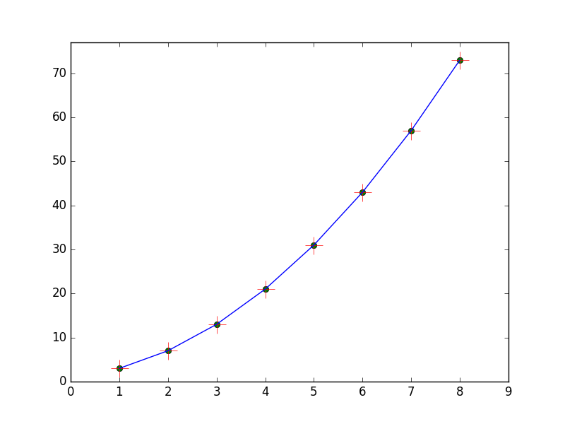
plt.plot(x, y, 'go')
plt.plot(x, interpolant(x), 'r+', markersize=18)
plt.plot(x, f(x), 'b')
plt.ylim(0, 77)
plt.xlim(0, 9)
plt.show()
程序执行结果:
12.4 runge龙格现象
一般来说,节点个数越多,插值函数和被插值函数就有越多的地方相等。但是随着插值节点个数的增加,两个插值节点之间插值函数并不一定能够很好地逼近被插值函数。再次,从舍入误差看,高次插值由于计算量大,可能会产生更严重的误差积累,所以,稳定性得不到保证。这就是Runge现象是龙格在研究多项式插值的时候,发现有的情况下,并非取节点(日期数)越多多项式就越精确。著名的例子是$f(x)=\frac{1}{1+25x^2}$,它的插值函数在两个端点处发生剧烈的波动,造成较大的误差。究其原因,是舍入误差造成的。解决Runge现象的方法是采用分段低次多项式插值:有分段线性插值和分段三次Hermite插值。在每个小区间采用低次插值,则可避免Runge现象。 龙格函数: $$ f(x)= \frac{1}{1 + 25x^2} $$ 下面看看重心坐标拉格郎日插值对龙格现象的处理效果。
from scipy.interpolate import BarycentricInterpolator,barycentric_interpolate, lagrange
import numpy as np
import numpy as np, matplotlib.pyplot as plt

nodes = np.linspace(-5, 5, 11)
x = np.linspace(-5,5,1000)

def f(t): return 1. / (1. + t**2)
interpolant = BarycentricInterpolator(nodes, f(nodes))

plt.subplot(121, aspect='auto')
plt.plot(x, interpolant(x), 'b--',label="Lagrange Interpolation")
plt.plot(nodes, f(nodes), 'ro', label='nodes')
plt.plot(x, f(x), 'r-', label="original")
plt.legend(loc=9)
plt.title("11 equally distributed nodes")


newnodes = np.linspace(-4.5, 4.5, 10)
interpolant.add_xi(newnodes, f(newnodes))
plt.subplot(122, aspect='auto')
plt.plot(x, interpolant(x), 'b--',label="Lagrange Interpolation")
plt.plot(nodes, f(nodes), 'ro', label='nodes')
plt.plot(x, f(x), 'r-', label="original")
plt.legend(loc=8)
plt.title("21 equally spaced nodes")
plt.show()
程序执行结果:
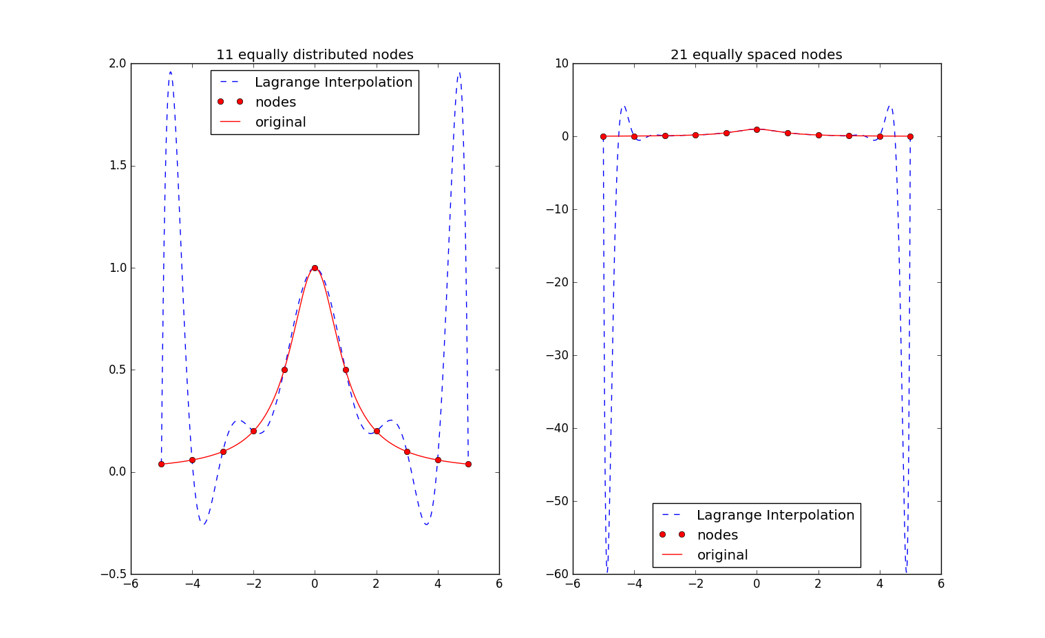 图中红色的是runge函数的可视化图形。从结果可以看出随着插值点的个数的增多,重心坐标插值法还算比较稳定的。
感谢Klang(金浪)智能数据看板klang.org.cn鼎力支持!