Python For Data Analysis-八章第三节
《Python For Data Analysis》的第八章的第三节主要讨论的是数据的变形问题涉及stack和unstack、pivot函数。
19.1 set_index函数生成层次化索引
在本Python学习网站的17章的第一节层次化索引生成的dataframe的层次化索引是通过给出相同的行名而产生的,在17章的最后去层次化索引一节提到了set_index函数,也给出了例子,这节继续使用set_index函数来构造层次化索引的dataframe,然后研究dataframe针对层次化的dataframe的的变形函数stack和unstack。
import pandas as pd
import numpy as np
tfboys = [['Donald Trump', 'English',65],['Donald Trump','Math',63],['Donald Trump','Politics',56],
          ['George.W.Bush', 'English',75],['George.W.Bush', 'Math',43],['George.W.Bush', 'Politics',36],
          ['William Clinton', 'English',55],['William Clinton', 'Math',58],['William Clinton', 'Politics',45]]
#print tfboys
df = pd.DataFrame(tfboys,columns = ["name", "course", "score"])
print "-" * 40
print df, "# df"
print "-" * 40
df.set_index(["name", "course"], inplace = True)
print df, "# df multiInde"
print "-" * 40
print df.index, “# df index”
print "-" * 40
执行结果:
----------------------------------------
              name    course  score
0     Donald Trump   English     65
1     Donald Trump      Math     63
2     Donald Trump  Politics     56
3    George.W.Bush   English     75
4    George.W.Bush      Math     43
5    George.W.Bush  Politics     36
6  William Clinton   English     55
7  William Clinton      Math     58
8  William Clinton  Politics     45 # df
----------------------------------------
                          score
name            course
Donald Trump    English      65
                Math         63
                Politics     56
George.W.Bush   English      75
                Math         43
                Politics     36
William Clinton English      55
                Math         58
                Politics     45 # df multiInde
----------------------------------------
MultiIndex(levels=[[u'Donald Trump', u'George.W.Bush', u'William Clinton'], [u'English', u'Math', u'Politics']],
           labels=[[0, 0, 0, 1, 1, 1, 2, 2, 2], [0, 1, 2, 0, 1, 2, 0, 1, 2]],
           names=[u'name', u'course'])# df index
----------------------------------------
set_index函数可以将多列设置为index即行索引,出现多层次的行索引。
19.2 stack函数和unstack函数
- stack函数可以将dataframe的列变行。
import pandas as pd
import numpy as np
tfboys = [['Donald Trump', 'English',65],['Donald Trump','Math',63],['Donald Trump','Politics',56],
          ['George.W.Bush', 'English',75],['George.W.Bush', 'Math',43],['George.W.Bush', 'Politics',36],
          ['William Clinton', 'English',55],['William Clinton', 'Math',58],['William Clinton', 'Politics',45]]
df = pd.DataFrame(tfboys,columns = ["name", "course", "score"])
print "-" * 40
print df, "# df"
print "-" * 40
df.set_index("name", inplace = True)
print df, "# df set_index"
print "-" * 40
print df.index, "# df.index"
print "-" * 40
print df.stack(), "# df stack()"
print "-" * 40
print df.stack().index, "# df stack() index"
print "-" * 40
执行结果:
----------------------------------------
              name    course  score
0     Donald Trump   English     65
1     Donald Trump      Math     63
2     Donald Trump  Politics     56
3    George.W.Bush   English     75
4    George.W.Bush      Math     43
5    George.W.Bush  Politics     36
6  William Clinton   English     55
7  William Clinton      Math     58
8  William Clinton  Politics     45 # df
----------------------------------------
                   course  score
name
Donald Trump      English     65
Donald Trump         Math     63
Donald Trump     Politics     56
George.W.Bush     English     75
George.W.Bush        Math     43
George.W.Bush    Politics     36
William Clinton   English     55
William Clinton      Math     58
William Clinton  Politics     45 # df set_index
----------------------------------------
Index([u'Donald Trump', u'Donald Trump', u'Donald Trump', u'George.W.Bush',
       u'George.W.Bush', u'George.W.Bush', u'William Clinton',
       u'William Clinton', u'William Clinton'],
      dtype='object', name=u'name') # df.index
----------------------------------------
name
Donald Trump     course     English
                 score           65
                 course        Math
                 score           63
                 course    Politics
                 score           56
George.W.Bush    course     English
                 score           75
                 course        Math
                 score           43
                 course    Politics
                 score           36
William Clinton  course     English
                 score           55
                 course        Math
                 score           58
                 course    Politics
                 score           45
dtype: object # df stack()
----------------------------------------
MultiIndex(levels=[[u'Donald Trump', u'George.W.Bush', u'William Clinton'], [u'course', u'score']],
           labels=[[0, 0, 0, 0, 0, 0, 1, 1, 1, 1, 1, 1, 2, 2, 2, 2, 2, 2], [0, 1, 0, 1, 0, 1, 0, 1, 0, 1, 0, 1, 0, 1, 0, 1, 0, 1]],
           names=[u'name', None]) # df stack() index
----------------------------------------
从stack函数的执行结果:
----------------------------------------
name
Donald Trump     course     English
                 score           65
                 course        Math
                 score           63
                 course    Politics
                 score           56
George.W.Bush    course     English
                 score           75
                 course        Math
                 score           43
                 course    Politics
                 score           36
William Clinton  course     English
                 score           55
                 course        Math
                 score           58
                 course    Politics
                 score           45
dtype: object # df stack()
----------------------------------------
MultiIndex(levels=[[u'Donald Trump', u'George.W.Bush', u'William Clinton'], [u'course', u'score']],
           labels=[[0, 0, 0, 0, 0, 0, 1, 1, 1, 1, 1, 1, 2, 2, 2, 2, 2, 2], [0, 1, 0, 1, 0, 1, 0, 1, 0, 1, 0, 1, 0, 1, 0, 1, 0, 1]],
           names=[u'name', None]) # df stack() index
----------------------------------------
可以看出stack也能产生层次化的多级的行索引。从print df.stack().index语句的输出结果:
----------------------------------------
MultiIndex(levels=[[u'Donald Trump', u'George.W.Bush', u'William Clinton'], [u'course', u'score']],
           labels=[[0, 0, 0, 0, 0, 0, 1, 1, 1, 1, 1, 1, 2, 2, 2, 2, 2, 2], [0, 1, 0, 1, 0, 1, 0, 1, 0, 1, 0, 1, 0, 1, 0, 1, 0, 1]],
           names=[u'name', None]) # df stack() index
----------------------------------------
也能看出是层次化多级索引。
- unstack函数可以将层次化索引的dataframe数据的行变列和stack正好相反。
import pandas as pd
import numpy as np
tfboys = [['Donald Trump', 'English',65],['Donald Trump','Math',63],['Donald Trump','Politics',56],
          ['George.W.Bush', 'English',75],['George.W.Bush', 'Math',43],['George.W.Bush', 'Politics',36],
          ['William Clinton', 'English',55],['William Clinton', 'Math',58],['William Clinton', 'Politics',45]]
df = pd.DataFrame(tfboys,columns = ["name", "course", "score"])
print "-" * 40
df.set_index("name", inplace = True)
df.columns.name = "info"
print df, "# df after set_index"
print "-" * 40
ret = df.stack()
print ret, "# df stack()"
print "-" * 40
print ret.unstack(), "# df stack() unstack()"
print "-" * 40
执行结果:
----------------------------------------
info               course  score
name
Donald Trump      English     65
...
William Clinton  Politics     45 # df after set_index
----------------------------------------
name             info
Donald Trump     course     English
                 score           65
                 course        Math
                 score           63
                 course    Politics
                 score           56
George.W.Bush    course     English
                 score           75
                 course        Math
                 score           43
                 course    Politics
                 score           36
William Clinton  course     English
                 score           55
                 course        Math
                 score           58
                 course    Politics
                 score           45
dtype: object # df stack()
----------------------------------------
Traceback (most recent call last):
  File "pda1901.py", line 15, in <module>
    print ret.unstack(), "# df stack() unstack()"
  File "/usr/local/lib/python2.7/dist-packages/pandas/core/series.py", line 2899, in unstack
    return unstack(self, level, fill_value)
  File "/usr/local/lib/python2.7/dist-packages/pandas/core/reshape/reshape.py", line 501, in unstack
    constructor=obj._constructor_expanddim)
  File "/usr/local/lib/python2.7/dist-packages/pandas/core/reshape/reshape.py", line 137, in __init__
    self._make_selectors()
  File "/usr/local/lib/python2.7/dist-packages/pandas/core/reshape/reshape.py", line 175, in _make_selectors
    raise ValueError('Index contains duplicate entries, '
ValueError: Index contains duplicate entries, cannot reshape
程序执行unstack函数的时候出现了错误ValueError: Index contains duplicate entries, cannot reshape说由于有重复数据无法reshape,重复数据在?
name             info
Donald Trump     course     English
                 score           65
                 course        Math
                 score           63
                 course    Politics
                 score           56
George.W.Bush    course     English
第二列info下有3个course和score原因是df.set_index("name", inplace = True)用name这一列做行索引,那么Donald Trump有三门课成绩,所以会在info有3个course和score。那怎么办?取消name做索引用自然整数(唯一不重复)。
import pandas as pd
import numpy as np
tfboys = [['Donald Trump', 'English',65],['Donald Trump','Math',63],['Donald Trump','Politics',56],
          ['George.W.Bush', 'English',75],['George.W.Bush', 'Math',43],['George.W.Bush', 'Politics',36],
          ['William Clinton', 'English',55],['William Clinton', 'Math',58],['William Clinton', 'Politics',45]]
df = pd.DataFrame(tfboys,columns = ["name", "course", "score"])
print "-" * 40
#df.set_index("name", inplace = True)
df.columns.name = "info"
print df, "# df after set_index"
print "-" * 40
ret = df.stack()
print ret, "# df stack()"
print "-" * 40
print ret.unstack(), "# df stack() unstack()"
print "-" * 40
执行结果:
----------------------------------------
info             name    course  score
0        Donald Trump   English     65
1        Donald Trump      Math     63
2        Donald Trump  Politics     56
3       George.W.Bush   English     75
4       George.W.Bush      Math     43
5       George.W.Bush  Politics     36
6     William Clinton   English     55
7     William Clinton      Math     58
8     William Clinton  Politics     45 # df after set_index
----------------------------------------
   info
0  name         Donald Trump
   course            English
   score                  65
1  name         Donald Trump
   course               Math
   score                  63
2  name         Donald Trump
   course           Politics
   score                  56
3  name        George.W.Bush
   course            English
   score                  75
4  name        George.W.Bush
   course               Math
   score                  43
5  name        George.W.Bush
   course           Politics
   score                  36
6  name      William Clinton
   course            English
   score                  55
7  name      William Clinton
   course               Math
   score                  58
8  name      William Clinton
   course           Politics
   score                  45
dtype: object # df stack()
----------------------------------------
info             name    course score
0        Donald Trump   English    65
1        Donald Trump      Math    63
2        Donald Trump  Politics    56
3       George.W.Bush   English    75
4       George.W.Bush      Math    43
5       George.W.Bush  Politics    36
6     William Clinton   English    55
7     William Clinton      Math    58
8     William Clinton  Politics    45 # df stack() unstack()
----------------------------------------
也就是层次化索引的dataframe如果能用unstack函数变回去,要求内层索引(此处是stack()后的info列)不能重复才能unstack。
19.3 pivot函数
pivot函数可以很轻松的构建出某种版式的透视表。数据透视表,是因为可以动态地改变它们的版面布置,以便按照不同方式分析数据,也可以重新安排行号、列标和页字段。每一次改变版面布置时,数据透视表会立即按照新的布置重新计算数据。另外,如果原始数据发生更改,则可以更新数据透视表。
19.3.1 JD股价数据
为了演示pivot函数的作用,可以先从Nasdaq下载JD的股票交易数据,进入该页面点击最下面的download下载股票历史交易记录,然后在看看pivot函数的作用。而这个数据在之前的Numpy部分的章节里有过接触过。
- Nasdaq网站JD股票交易数据网址

- JD交易数据网站展示
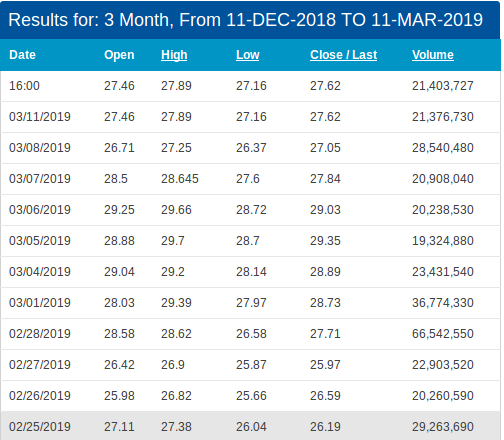
- 下载的文件:HistoricalQuotes文件的格式是csv的,如下图:

- 读取数据文,HistoricalQuotes.csv文件和下面的代码保存在同一个目录下,这个下载的数据文件是.csv的类型文件,可以用之前学习过的一些函数读取这个文件到dataframe里,这里可以使用read_table函数。
import pandas as pd
import numpy as np
from pandas.tseries.offsets import DateOffset
df = pd.read_table("HistoricalQuotes.csv", sep = ",")
print "-" * 60
print df[:10], "# after read_table"
print "-" * 60
执行结果:
------------------------------------------------------------
         date  close      volume   open    high    low
0  2019/03/11  27.62  21376730.0  27.46  27.890  27.16
1  2019/03/08  27.05  28540480.0  26.71  27.250  26.37
2  2019/03/07  27.84  20908040.0  28.50  28.645  27.60
3  2019/03/06  29.03  20238530.0  29.25  29.660  28.72
4  2019/03/05  29.35  19324880.0  28.88  29.700  28.70
5  2019/03/04  28.89  23431540.0  29.04  29.200  28.14
6  2019/03/01  28.73  36774330.0  28.03  29.390  27.97
7  2019/02/28  27.71  66542550.0  28.58  28.620  26.58
8  2019/02/27  25.97  22903520.0  26.42  26.900  25.87
9  2019/02/26  26.59  20260590.0  25.98  26.820  25.66 # after read_table
------------------------------------------------------------
从执行结果可以看出,数据文件里有若干列,分别记录交易日期、收盘价、交易量、开盘价、最高交易价和最低交易价这些数据。
19.3.2 JD股票数据透视表
之前一小节可以成功下载、读取数据文件数据到dataframe里了,这节要解决的问题是对数据进行必要的变形、变化,调整成便于分析统计的样式。暂不使用pivot,看已学的其他函数能不能实现pivot函数的作用。
1). 数据逆序
可以自行打开HistoricalQuotes.csv数据文件查看一下,发现最新的交易时间在第一行,而久远的交易时间在最后一行,我们想调整一下按时间先后顺序排列,而不是倒序,此时的df的行索引是整数的有序增大,所以可以使用sort_index函数来逆序一下整个数据。
import pandas as pd
import numpy as np
from pandas.tseries.offsets import DateOffset
df = pd.read_table("HistoricalQuotes.csv", sep = ",")
print "-" * 60
print df[:10], "# after read_table"

df.sort_index(ascending=False, inplace=True)
print "-" * 60
print df[:10], "# after sort on index"
print "-" * 60
执行结果:
------------------------------------------------------------
         date  close      volume   open    high    low
0  2019/03/11  27.62  21376730.0  27.46  27.890  27.16
1  2019/03/08  27.05  28540480.0  26.71  27.250  26.37
2  2019/03/07  27.84  20908040.0  28.50  28.645  27.60
3  2019/03/06  29.03  20238530.0  29.25  29.660  28.72
4  2019/03/05  29.35  19324880.0  28.88  29.700  28.70
5  2019/03/04  28.89  23431540.0  29.04  29.200  28.14
6  2019/03/01  28.73  36774330.0  28.03  29.390  27.97
7  2019/02/28  27.71  66542550.0  28.58  28.620  26.58
8  2019/02/27  25.97  22903520.0  26.42  26.900  25.87
9  2019/02/26  26.59  20260590.0  25.98  26.820  25.66 # after read_table
------------------------------------------------------------
          date  close      volume   open     high    low
60  2018/12/11  20.91  13234290.0  20.95  21.3400  20.82
59  2018/12/12  21.89  19641470.0  21.30  22.3150  21.27
58  2018/12/13  22.71  25465660.0  22.00  23.3500  22.00
57  2018/12/14  22.17  14866570.0  22.04  22.9400  22.01
56  2018/12/17  21.35  16522610.0  22.04  22.2600  21.17
55  2018/12/18  21.04  14253720.0  21.47  21.8369  20.91
54  2018/12/19  20.17  15254470.0  20.95  21.4850  20.00
53  2018/12/20  19.91  17855170.0  20.09  20.2100  19.64
52  2018/12/21  21.08  49463160.0  20.09  21.9900  19.52
51  2018/12/24  19.75  28037350.0  21.49  21.5100  19.26 # after sort on index
------------------------------------------------------------
df里的数据按date即交易时间逆序了,即现在的df的第一条数据是最早的交易时间了,可能比较符合一般人观察习惯。
2). 用交易时间做行索引
如果不打算用整数作为每条数据的数据可以使用set_index函数来指定某列为新生成的dataframe的行索引。
import pandas as pd
import numpy as np
from pandas.tseries.offsets import DateOffset
df = pd.read_table("HistoricalQuotes.csv", sep = ",")
print "-" * 60
print df[:10], "# after read_table"

df.sort_index(ascending=False, inplace=True)
print "-" * 60
print df[:10], "# after sort on index"
print "-" * 60
print df.set_index("date")[:10], "# after set index on date"
print "-" * 60
执行结果:
------------------------------------------------------------
         date  close      volume   open    high    low
0  2019/03/11  27.62  21376730.0  27.46  27.890  27.16
1  2019/03/08  27.05  28540480.0  26.71  27.250  26.37
2  2019/03/07  27.84  20908040.0  28.50  28.645  27.60
3  2019/03/06  29.03  20238530.0  29.25  29.660  28.72
4  2019/03/05  29.35  19324880.0  28.88  29.700  28.70
5  2019/03/04  28.89  23431540.0  29.04  29.200  28.14
6  2019/03/01  28.73  36774330.0  28.03  29.390  27.97
7  2019/02/28  27.71  66542550.0  28.58  28.620  26.58
8  2019/02/27  25.97  22903520.0  26.42  26.900  25.87
9  2019/02/26  26.59  20260590.0  25.98  26.820  25.66 # after read_table
------------------------------------------------------------
          date  close      volume   open     high    low
60  2018/12/11  20.91  13234290.0  20.95  21.3400  20.82
59  2018/12/12  21.89  19641470.0  21.30  22.3150  21.27
58  2018/12/13  22.71  25465660.0  22.00  23.3500  22.00
57  2018/12/14  22.17  14866570.0  22.04  22.9400  22.01
56  2018/12/17  21.35  16522610.0  22.04  22.2600  21.17
55  2018/12/18  21.04  14253720.0  21.47  21.8369  20.91
54  2018/12/19  20.17  15254470.0  20.95  21.4850  20.00
53  2018/12/20  19.91  17855170.0  20.09  20.2100  19.64
52  2018/12/21  21.08  49463160.0  20.09  21.9900  19.52
51  2018/12/24  19.75  28037350.0  21.49  21.5100  19.26 # after sort on index
------------------------------------------------------------
            close      volume   open     high    low
date
2018/12/11  20.91  13234290.0  20.95  21.3400  20.82
2018/12/12  21.89  19641470.0  21.30  22.3150  21.27
2018/12/13  22.71  25465660.0  22.00  23.3500  22.00
2018/12/14  22.17  14866570.0  22.04  22.9400  22.01
2018/12/17  21.35  16522610.0  22.04  22.2600  21.17
2018/12/18  21.04  14253720.0  21.47  21.8369  20.91
2018/12/19  20.17  15254470.0  20.95  21.4850  20.00
2018/12/20  19.91  17855170.0  20.09  20.2100  19.64
2018/12/21  21.08  49463160.0  20.09  21.9900  19.52
2018/12/24  19.75  28037350.0  21.49  21.5100  19.26 # after set index on date
------------------------------------------------------------
这也许是某些数据分析师分析数据时所想要的内容。
3). 构建周开盘闭盘时间
此时的数据是每天都有,如果只想关心JD股票每周周一股市开盘、和周五股市闭盘的情况,那么需要对date列的数据进行过滤,即只保留周一和周五的时间,如何做?
import pandas as pd
import numpy as np
from pandas.tseries.offsets import DateOffset
df = pd.read_table("HistoricalQuotes.csv", sep = ",")
print "-" * 60
print df[:10], "# after read_table"
df.sort_index(ascending=False, inplace=True)
print "-" * 60
print df[:10], "# after sort on index"
print "-" * 60
st = pd.Timestamp(df.iloc[0, 0])
date_mon = pd.date_range(start= st,end = st + DateOffset(months=3),freq='W-MON')
date_fri = pd.date_range(start= st,end = st + DateOffset(months=3),freq='W-FRI')
exchange_day = date_mon.union(date_fri)
print exchange_day, "# exchange_day"
sel_day = exchange_day.strftime("%Y/%m/%d")
print "-" * 60
print sel_day, "# sel_day"
print "-" * 60
执行结果:
------------------------------------------------------------
         date  close      volume   open    high    low
0  2019/03/11  27.62  21376730.0  27.46  27.890  27.16
1  2019/03/08  27.05  28540480.0  26.71  27.250  26.37
2  2019/03/07  27.84  20908040.0  28.50  28.645  27.60
3  2019/03/06  29.03  20238530.0  29.25  29.660  28.72
4  2019/03/05  29.35  19324880.0  28.88  29.700  28.70
5  2019/03/04  28.89  23431540.0  29.04  29.200  28.14
6  2019/03/01  28.73  36774330.0  28.03  29.390  27.97
7  2019/02/28  27.71  66542550.0  28.58  28.620  26.58
8  2019/02/27  25.97  22903520.0  26.42  26.900  25.87
9  2019/02/26  26.59  20260590.0  25.98  26.820  25.66 # after read_table
------------------------------------------------------------
          date  close      volume   open     high    low
60  2018/12/11  20.91  13234290.0  20.95  21.3400  20.82
59  2018/12/12  21.89  19641470.0  21.30  22.3150  21.27
58  2018/12/13  22.71  25465660.0  22.00  23.3500  22.00
57  2018/12/14  22.17  14866570.0  22.04  22.9400  22.01
56  2018/12/17  21.35  16522610.0  22.04  22.2600  21.17
55  2018/12/18  21.04  14253720.0  21.47  21.8369  20.91
54  2018/12/19  20.17  15254470.0  20.95  21.4850  20.00
53  2018/12/20  19.91  17855170.0  20.09  20.2100  19.64
52  2018/12/21  21.08  49463160.0  20.09  21.9900  19.52
51  2018/12/24  19.75  28037350.0  21.49  21.5100  19.26 # after sort on index
------------------------------------------------------------
DatetimeIndex(['2018-12-14', '2018-12-17', '2018-12-21', '2018-12-24',
               '2018-12-28', '2018-12-31', '2019-01-04', '2019-01-07',
               '2019-01-11', '2019-01-14', '2019-01-18', '2019-01-21',
               '2019-01-25', '2019-01-28', '2019-02-01', '2019-02-04',
               '2019-02-08', '2019-02-11', '2019-02-15', '2019-02-18',
               '2019-02-22', '2019-02-25', '2019-03-01', '2019-03-04',
               '2019-03-08', '2019-03-11'],
              dtype='datetime64[ns]', freq=None) # exchange_day
------------------------------------------------------------
Index([u'2018/12/14', u'2018/12/17', u'2018/12/21', u'2018/12/24',
       u'2018/12/28', u'2018/12/31', u'2019/01/04', u'2019/01/07',
       u'2019/01/11', u'2019/01/14', u'2019/01/18', u'2019/01/21',
       u'2019/01/25', u'2019/01/28', u'2019/02/01', u'2019/02/04',
       u'2019/02/08', u'2019/02/11', u'2019/02/15', u'2019/02/18',
       u'2019/02/22', u'2019/02/25', u'2019/03/01', u'2019/03/04',
       u'2019/03/08', u'2019/03/11'],
      dtype='object') #sel_day
------------------------------------------------------------
变量exchange_day里是周一和周五的时间数据。使用的range_date函数在时间序列的创建一章和data_range参数两节介绍过。
由于date_range函数产生的时间序列是DateTimeIndex类型的,不能直接被DataFrame通过loc来提取以以时间作为行索引的数据行,所以需要对exchange_day(类型为DatetimeIndex)进行数据类型的转换得到sel_day(类型为Index)。
4). 提取若干列数据
JD的股票交易数据文件HistoricalQuotes.csv有若干列,如果只关注其中几列的数据,如交易量、最高和最低交易价,可以使用reindex函数的columns参数来提取、限定数据列的输出。
import pandas as pd
import numpy as np
from pandas.tseries.offsets import DateOffset
df = pd.read_table("HistoricalQuotes.csv", sep = ",")
print "-" * 60
print df[:10], "# after read_table"
df.sort_index(ascending=False, inplace=True)
print "-" * 60
print df[:10], "# after sort on index"
print "-" * 60
st = pd.Timestamp(df.iloc[0, 0])
date_mon = pd.date_range(start= st,end = st + DateOffset(months=3),freq='W-MON')
date_fri = pd.date_range(start= st,end = st + DateOffset(months=3),freq='W-FRI')
exchange_day = date_mon.union(date_fri)
#print exchange_day, "# exchange_day"
sel_day = exchange_day.strftime("%Y/%m/%d")
#print "-" * 60
#print sel_day, "sel_day"
#print "-" * 60
cols = pd.Index(['date', 'volume', 'high','low'], name='item')
print cols, "# index on columns"
print "-" * 60
dd = df.reindex(columns = cols)
print dd[:10], "# reindex to get some columns"
print "-" * 60
执行结果:
------------------------------------------------------------
         date  close      volume   open    high    low
0  2019/03/11  27.62  21376730.0  27.46  27.890  27.16
1  2019/03/08  27.05  28540480.0  26.71  27.250  26.37
2  2019/03/07  27.84  20908040.0  28.50  28.645  27.60
3  2019/03/06  29.03  20238530.0  29.25  29.660  28.72
4  2019/03/05  29.35  19324880.0  28.88  29.700  28.70
5  2019/03/04  28.89  23431540.0  29.04  29.200  28.14
6  2019/03/01  28.73  36774330.0  28.03  29.390  27.97
7  2019/02/28  27.71  66542550.0  28.58  28.620  26.58
8  2019/02/27  25.97  22903520.0  26.42  26.900  25.87
9  2019/02/26  26.59  20260590.0  25.98  26.820  25.66 # after read_table
------------------------------------------------------------
          date  close      volume   open     high    low
60  2018/12/11  20.91  13234290.0  20.95  21.3400  20.82
59  2018/12/12  21.89  19641470.0  21.30  22.3150  21.27
58  2018/12/13  22.71  25465660.0  22.00  23.3500  22.00
57  2018/12/14  22.17  14866570.0  22.04  22.9400  22.01
56  2018/12/17  21.35  16522610.0  22.04  22.2600  21.17
55  2018/12/18  21.04  14253720.0  21.47  21.8369  20.91
54  2018/12/19  20.17  15254470.0  20.95  21.4850  20.00
53  2018/12/20  19.91  17855170.0  20.09  20.2100  19.64
52  2018/12/21  21.08  49463160.0  20.09  21.9900  19.52
51  2018/12/24  19.75  28037350.0  21.49  21.5100  19.26 # after sort on index
------------------------------------------------------------
Index([u'date', u'volume', u'high', u'low'], dtype='object', name=u'item') # index on columns
------------------------------------------------------------
item        date      volume     high    low
60    2018/12/11  13234290.0  21.3400  20.82
59    2018/12/12  19641470.0  22.3150  21.27
58    2018/12/13  25465660.0  23.3500  22.00
57    2018/12/14  14866570.0  22.9400  22.01
56    2018/12/17  16522610.0  22.2600  21.17
55    2018/12/18  14253720.0  21.8369  20.91
54    2018/12/19  15254470.0  21.4850  20.00
53    2018/12/20  17855170.0  20.2100  19.64
52    2018/12/21  49463160.0  21.9900  19.52
51    2018/12/24  28037350.0  21.5100  19.26 # reindex to get some columns
------------------------------------------------------------
从dd = df.reindex(columns = cols)语句的执行结果可以看到,只提取了原数据文件里的四列数据date、volume、high、low。
5). 指定date为索引
现在想用date列作为行索引而不是用默认的整形数据做行索引。
import pandas as pd
import numpy as np
from pandas.tseries.offsets import DateOffset
df = pd.read_table("HistoricalQuotes.csv", sep = ",")
print "-" * 60
print df[:10], "# after read_table"
df.sort_index(ascending=False, inplace=True)
print "-" * 60
print df[:10], "# after sort on index"
print "-" * 60
st = pd.Timestamp(df.iloc[0, 0])
date_mon = pd.date_range(start= st,end = st + DateOffset(months=3),freq='W-MON')
date_fri = pd.date_range(start= st,end = st + DateOffset(months=3),freq='W-FRI')
exchange_day = date_mon.union(date_fri)
#print exchange_day, "# exchange_day"
sel_day = exchange_day.strftime("%Y/%m/%d")
#print "-" * 60
#print sel_day, "sel_day"
#print "-" * 60
cols = pd.Index(['date', 'volume', 'high','low'], name='item')
#print cols, "# index on columns"
#print "-" * 60
dd = df.reindex(columns = cols)
print dd[:10], "# reindex to get some columns"
print "-" * 60
dd = df.reindex(columns = cols).set_index("date")
print dd[:10], "# reindex set_index ond date"
print "-" * 60
执行结果:
------------------------------------------------------------
         date  close      volume   open    high    low
0  2019/03/11  27.62  21376730.0  27.46  27.890  27.16
1  2019/03/08  27.05  28540480.0  26.71  27.250  26.37
2  2019/03/07  27.84  20908040.0  28.50  28.645  27.60
3  2019/03/06  29.03  20238530.0  29.25  29.660  28.72
4  2019/03/05  29.35  19324880.0  28.88  29.700  28.70
5  2019/03/04  28.89  23431540.0  29.04  29.200  28.14
6  2019/03/01  28.73  36774330.0  28.03  29.390  27.97
7  2019/02/28  27.71  66542550.0  28.58  28.620  26.58
8  2019/02/27  25.97  22903520.0  26.42  26.900  25.87
9  2019/02/26  26.59  20260590.0  25.98  26.820  25.66 # after read_table
------------------------------------------------------------
          date  close      volume   open     high    low
60  2018/12/11  20.91  13234290.0  20.95  21.3400  20.82
59  2018/12/12  21.89  19641470.0  21.30  22.3150  21.27
58  2018/12/13  22.71  25465660.0  22.00  23.3500  22.00
57  2018/12/14  22.17  14866570.0  22.04  22.9400  22.01
56  2018/12/17  21.35  16522610.0  22.04  22.2600  21.17
55  2018/12/18  21.04  14253720.0  21.47  21.8369  20.91
54  2018/12/19  20.17  15254470.0  20.95  21.4850  20.00
53  2018/12/20  19.91  17855170.0  20.09  20.2100  19.64
52  2018/12/21  21.08  49463160.0  20.09  21.9900  19.52
51  2018/12/24  19.75  28037350.0  21.49  21.5100  19.26 # after sort on index
------------------------------------------------------------
item        date      volume     high    low
60    2018/12/11  13234290.0  21.3400  20.82
59    2018/12/12  19641470.0  22.3150  21.27
58    2018/12/13  25465660.0  23.3500  22.00
57    2018/12/14  14866570.0  22.9400  22.01
56    2018/12/17  16522610.0  22.2600  21.17
55    2018/12/18  14253720.0  21.8369  20.91
54    2018/12/19  15254470.0  21.4850  20.00
53    2018/12/20  17855170.0  20.2100  19.64
52    2018/12/21  49463160.0  21.9900  19.52
51    2018/12/24  28037350.0  21.5100  19.26 # reindex to get some columns
------------------------------------------------------------
item            volume     high    low
date
2018/12/11  13234290.0  21.3400  20.82
2018/12/12  19641470.0  22.3150  21.27
2018/12/13  25465660.0  23.3500  22.00
2018/12/14  14866570.0  22.9400  22.01
2018/12/17  16522610.0  22.2600  21.17
2018/12/18  14253720.0  21.8369  20.91
2018/12/19  15254470.0  21.4850  20.00
2018/12/20  17855170.0  20.2100  19.64
2018/12/21  49463160.0  21.9900  19.52
2018/12/24  28037350.0  21.5100  19.26 # reindex set_index ond date
------------------------------------------------------------
6). 提取周一开盘和周五闭市交易数据
这个时候可以用之前3). 构建周开盘闭盘时间里的sel_day的周一和周五的时间序列来提取只有周一和周五的数据交易信息了。
import pandas as pd
import numpy as np
from pandas.tseries.offsets import DateOffset
df = pd.read_table("HistoricalQuotes.csv", sep = ",")
print "-" * 60
print df[:10], "# after read_table"
df.sort_index(ascending=False, inplace=True)
print "-" * 60
print df[:10], "# after sort on index"
print "-" * 60
st = pd.Timestamp(df.iloc[0, 0])
date_mon = pd.date_range(start= st,end = st + DateOffset(months=3),freq='W-MON')
date_fri = pd.date_range(start= st,end = st + DateOffset(months=3),freq='W-FRI')
exchange_day = date_mon.union(date_fri)
#print exchange_day, "# exchange_day"
sel_day = exchange_day.strftime("%Y/%m/%d")
#print "-" * 60
#print sel_day, "sel_day"
#print "-" * 60
cols = pd.Index(['date', 'volume', 'high','low'], name='item')
#print cols, "# index on columns"
#print "-" * 60
dd = df.reindex(columns = cols)
print dd[:10], "# reindex to get some columns"
print "-" * 60
dd = df.reindex(columns = cols).set_index("date").loc[sel_day]
print dd, "# select Monday and Friday"
print "-" * 60
执行结果:
------------------------------------------------------------
         date  close      volume   open    high    low
0  2019/03/11  27.62  21376730.0  27.46  27.890  27.16
1  2019/03/08  27.05  28540480.0  26.71  27.250  26.37
2  2019/03/07  27.84  20908040.0  28.50  28.645  27.60
3  2019/03/06  29.03  20238530.0  29.25  29.660  28.72
4  2019/03/05  29.35  19324880.0  28.88  29.700  28.70
5  2019/03/04  28.89  23431540.0  29.04  29.200  28.14
6  2019/03/01  28.73  36774330.0  28.03  29.390  27.97
7  2019/02/28  27.71  66542550.0  28.58  28.620  26.58
8  2019/02/27  25.97  22903520.0  26.42  26.900  25.87
9  2019/02/26  26.59  20260590.0  25.98  26.820  25.66 # after read_table
------------------------------------------------------------
          date  close      volume   open     high    low
60  2018/12/11  20.91  13234290.0  20.95  21.3400  20.82
59  2018/12/12  21.89  19641470.0  21.30  22.3150  21.27
58  2018/12/13  22.71  25465660.0  22.00  23.3500  22.00
57  2018/12/14  22.17  14866570.0  22.04  22.9400  22.01
56  2018/12/17  21.35  16522610.0  22.04  22.2600  21.17
55  2018/12/18  21.04  14253720.0  21.47  21.8369  20.91
54  2018/12/19  20.17  15254470.0  20.95  21.4850  20.00
53  2018/12/20  19.91  17855170.0  20.09  20.2100  19.64
52  2018/12/21  21.08  49463160.0  20.09  21.9900  19.52
51  2018/12/24  19.75  28037350.0  21.49  21.5100  19.26 # after sort on index
------------------------------------------------------------
item        date      volume     high    low
60    2018/12/11  13234290.0  21.3400  20.82
59    2018/12/12  19641470.0  22.3150  21.27
58    2018/12/13  25465660.0  23.3500  22.00
57    2018/12/14  14866570.0  22.9400  22.01
56    2018/12/17  16522610.0  22.2600  21.17
55    2018/12/18  14253720.0  21.8369  20.91
54    2018/12/19  15254470.0  21.4850  20.00
53    2018/12/20  17855170.0  20.2100  19.64
52    2018/12/21  49463160.0  21.9900  19.52
51    2018/12/24  28037350.0  21.5100  19.26 # reindex to get some columns
------------------------------------------------------------
item            volume     high      low
2018/12/14  14866570.0  22.9400  22.0100
2018/12/17  16522610.0  22.2600  21.1700
2018/12/21  49463160.0  21.9900  19.5200
2018/12/24  28037350.0  21.5100  19.2600
2018/12/28  16629620.0  22.0000  21.1500
2018/12/31  19407160.0  22.4800  20.7700
2019/01/04  25132510.0  22.6800  20.7501
2019/01/07  18843420.0  22.8500  22.2600
2019/01/11  10017400.0  23.7500  22.6900
2019/01/14  14120930.0  22.3000  21.5300
2019/01/18  23260730.0  23.8500  22.3000
2019/01/21         NaN      NaN      NaN
2019/01/25  28015970.0  23.9300  22.4700
2019/01/28  13884910.0  24.1399  23.0600
2019/02/01  11928890.0  25.3100  24.3100
2019/02/04   9046348.0  24.5400  24.1600
2019/02/08   8239639.0  24.2800  23.6000
2019/02/11   9025630.0  24.7300  24.1500
2019/02/15  11468160.0  24.5700  23.9100
2019/02/18         NaN      NaN      NaN
2019/02/22  27084030.0  25.9600  24.4800
2019/02/25  29263690.0  27.3800  26.0400
2019/03/01  36774330.0  29.3900  27.9700
2019/03/04  23431540.0  29.2000  28.1400
2019/03/08  28540480.0  27.2500  26.3700
2019/03/11  21376730.0  27.8900  27.1600 # select Monday and Friday
------------------------------------------------------------
7). 按日查看数据信息,可以使用stack函数创建层次化的索引能满足需求。
import pandas as pd
import numpy as np
from pandas.tseries.offsets import DateOffset
df = pd.read_table("HistoricalQuotes.csv", sep = ",")
print "-" * 60
print df[:10], "# after read_table"
df.sort_index(ascending=False, inplace=True)
#print "-" * 60
#print df[:10], "# after sort on index"
#print "-" * 60
st = pd.Timestamp(df.iloc[0, 0])
date_mon = pd.date_range(start= st,end = st + DateOffset(months=3),freq='W-MON')
date_fri = pd.date_range(start= st,end = st + DateOffset(months=3),freq='W-FRI')
exchange_day = date_mon.union(date_fri)
#print exchange_day, "# exchange_day"
sel_day = exchange_day.strftime("%Y/%m/%d")
#print "-" * 60
#print sel_day, "sel_day"
#print "-" * 60
cols = pd.Index(['date', 'volume', 'high','low'], name='item')
#print cols, "# index on columns"
#print "-" * 60
dd = df.reindex(columns = cols)
#print dd[:10], "# reindex to get some columns"
#print "-" * 60
dd = df.reindex(columns = cols).set_index("date").loc[sel_day]
#print dd, "# select Monday and Friday"
print "-" * 60
print dd.stack(), "# stack"
最后的输出是按日期输出的当日交易量、最高价和最低交易价信息,执行结果:
------------------------------------------------------------
         date  close      volume   open    high    low
0  2019/03/11  27.62  21376730.0  27.46  27.890  27.16
1  2019/03/08  27.05  28540480.0  26.71  27.250  26.37
2  2019/03/07  27.84  20908040.0  28.50  28.645  27.60
3  2019/03/06  29.03  20238530.0  29.25  29.660  28.72
4  2019/03/05  29.35  19324880.0  28.88  29.700  28.70
5  2019/03/04  28.89  23431540.0  29.04  29.200  28.14
6  2019/03/01  28.73  36774330.0  28.03  29.390  27.97
7  2019/02/28  27.71  66542550.0  28.58  28.620  26.58
8  2019/02/27  25.97  22903520.0  26.42  26.900  25.87
9  2019/02/26  26.59  20260590.0  25.98  26.820  25.66 # after read_table
------------------------------------------------------------
            item
2018/12/14  volume    1.486657e+07
            high      2.294000e+01
            low       2.201000e+01
2018/12/17  volume    1.652261e+07
            high      2.226000e+01
            low       2.117000e+01
...<中间部分省略>....
2019/03/08  volume    2.854048e+07
            high      2.725000e+01
            low       2.637000e+01
2019/03/11  volume    2.137673e+07
            high      2.789000e+01
            low       2.716000e+01
Length: 72, dtype: float64 # stack
19.3.3 pivot函数
这一小节,使用pivot来作出上一小节的数据透视表的效果。
import pandas as pd
import numpy as np
from pandas.tseries.offsets import DateOffset
df = pd.read_table("HistoricalQuotes.csv", sep = ",")
print "-" * 60
print df[:10], "# after read_table"
df.sort_index(ascending=False, inplace=True)
st = pd.Timestamp(df.iloc[0, 0])
date_mon = pd.date_range(start= st,end = st + DateOffset(months=3),freq='W-MON')
date_fri = pd.date_range(start= st,end = st + DateOffset(months=3),freq='W-FRI')
exchange_day = date_mon.union(date_fri)
sel_day = exchange_day.strftime("%Y/%m/%d")
cols = pd.Index(['date', 'volume', 'high','low'], name='item')
dd = df.reindex(columns = cols).set_index("date").stack()
print "-" * 60
print dd[:10], "# stack"
print "-" * 60
dd = dd.reset_index()
print dd[:10], "# reset index"
print "-" * 60
dd =  dd.rename(columns={0: 'value'})
print dd[:10], "# rename"
p = dd.pivot('date', 'item', 'value')
print "-" * 60
print p.loc[sel_day], "# pivot"
print "-" * 60
执行结果:
------------------------------------------------------------
         date  close      volume   open    high    low
0  2019/03/11  27.62  21376730.0  27.46  27.890  27.16
1  2019/03/08  27.05  28540480.0  26.71  27.250  26.37
2  2019/03/07  27.84  20908040.0  28.50  28.645  27.60
3  2019/03/06  29.03  20238530.0  29.25  29.660  28.72
4  2019/03/05  29.35  19324880.0  28.88  29.700  28.70
5  2019/03/04  28.89  23431540.0  29.04  29.200  28.14
6  2019/03/01  28.73  36774330.0  28.03  29.390  27.97
7  2019/02/28  27.71  66542550.0  28.58  28.620  26.58
8  2019/02/27  25.97  22903520.0  26.42  26.900  25.87
9  2019/02/26  26.59  20260590.0  25.98  26.820  25.66 # after read_table
------------------------------------------------------------
date        item
2018/12/11  volume    1.323429e+07
            high      2.134000e+01
            low       2.082000e+01
2018/12/12  volume    1.964147e+07
            high      2.231500e+01
            low       2.127000e+01
2018/12/13  volume    2.546566e+07
            high      2.335000e+01
            low       2.200000e+01
2018/12/14  volume    1.486657e+07
dtype: float64 # stack
------------------------------------------------------------
         date    item             0
0  2018/12/11  volume  1.323429e+07
1  2018/12/11    high  2.134000e+01
2  2018/12/11     low  2.082000e+01
3  2018/12/12  volume  1.964147e+07
4  2018/12/12    high  2.231500e+01
5  2018/12/12     low  2.127000e+01
6  2018/12/13  volume  2.546566e+07
7  2018/12/13    high  2.335000e+01
8  2018/12/13     low  2.200000e+01
9  2018/12/14  volume  1.486657e+07 # reset index
------------------------------------------------------------
         date    item         value
0  2018/12/11  volume  1.323429e+07
1  2018/12/11    high  2.134000e+01
2  2018/12/11     low  2.082000e+01
3  2018/12/12  volume  1.964147e+07
4  2018/12/12    high  2.231500e+01
5  2018/12/12     low  2.127000e+01
6  2018/12/13  volume  2.546566e+07
7  2018/12/13    high  2.335000e+01
8  2018/12/13     low  2.200000e+01
9  2018/12/14  volume  1.486657e+07 # rename
------------------------------------------------------------
item           high      low      volume
2018/12/14  22.9400  22.0100  14866570.0
2018/12/17  22.2600  21.1700  16522610.0
2018/12/21  21.9900  19.5200  49463160.0
2018/12/24  21.5100  19.2600  28037350.0
2018/12/28  22.0000  21.1500  16629620.0
2018/12/31  22.4800  20.7700  19407160.0
2019/01/04  22.6800  20.7501  25132510.0
2019/01/07  22.8500  22.2600  18843420.0
2019/01/11  23.7500  22.6900  10017400.0
2019/01/14  22.3000  21.5300  14120930.0
2019/01/18  23.8500  22.3000  23260730.0
2019/01/21      NaN      NaN         NaN
2019/01/25  23.9300  22.4700  28015970.0
2019/01/28  24.1399  23.0600  13884910.0
2019/02/01  25.3100  24.3100  11928890.0
2019/02/04  24.5400  24.1600   9046348.0
2019/02/08  24.2800  23.6000   8239639.0
2019/02/11  24.7300  24.1500   9025630.0
2019/02/15  24.5700  23.9100  11468160.0
2019/02/18      NaN      NaN         NaN
2019/02/22  25.9600  24.4800  27084030.0
2019/02/25  27.3800  26.0400  29263690.0
2019/03/01  29.3900  27.9700  36774330.0
2019/03/04  29.2000  28.1400  23431540.0
2019/03/08  27.2500  26.3700  28540480.0
2019/03/11  27.8900  27.1600  21376730.0 # pivot
------------------------------------------------------------
两小节的区别是,上一小节的6). 提取周一开盘和周五闭市交易数据是通过将索引设置为date列为索引的到
------------------------------------------------------------
item            volume     high      low
2018/12/14  14866570.0  22.9400  22.0100
....
2019/03/11  21376730.0  27.8900  27.1600 # select Monday and Friday
------------------------------------------------------------
结果的,而本小节则是通过stack层次化索引和reset_index去层次化索引增加整数作为行索引之后用pivot得到这个结果。
感谢Klang(金浪)智能数据看板klang.org.cn鼎力支持!